Optimization Project: Part I

Overview
Optimization is one of the most powerful and flexible methods of quantitative analysis. One type of optimization is linear programming (LP). Linear programming is used on a daily basis to solve a wide variety of problems. These problems include inventory management, bond trading, cash flow management, and staffing. Linear programming problems involve optimizing a linear function subject to constraints. These constraints are expressed as linear inequalities or equalities. Linear programming is based on the simplex method, developed by George Dantzig. The method involves a systematic, arithmetic-intensive search through the set of all possible solutions for the solution that optimizes a specific objective. To date, this is the most important solution method for linear programming models.

Understanding Linear Programming Concepts
Two ways to formulate a linear programming model include:

1. Algebraic Formulation (traditional)

2. Spreadsheet Formulation (modern)

Algebraic Formulation: In the traditional algebraic solution method, the decision variables are identified first. Second, the objective and constraints are written in terms of the decision variable label (e.g. x_1, x_2, x_3, x_4). Third, explicit constraints are added to ensure that the variables are nonnegative.

Spreadsheet Formulation: In the past, all LP problems were formulated algebraically. As a result, many commercial LP computer applications are written to accept LP problems in this format. The LINDO package is one example. Newer methods incorporate a more intuitive method of expressing LP problems. With the availability of Solver add-ins, spreadsheets now have the capability of formulating and optimizing (solving) LP problems. Applications that have built-in Solvers include Microsoft Excel, Lotus 1-2-3, and Corel Quattro Pro.

Common spreadsheet elements in LP models are:

1. Inputs – The data needed to form the objective and constraints.

2. Changing Cells – Designated cells that play the role of the decision variables that can be changed to optimize the objective.

3. Target Cell (Objective) – Cell that contains the value of the objective.

4. Constraints – Statements specified in the Solver dialog box.

5. Nonnegativity – Specified by checking a box to indicate nonnegative changing cells (decision variables).

The solution of a LP problem involves three (3) stages. They are:

1. Enter all inputs, trial values for the changing cells and related formulas in a spreadsheet.

2. Invoke Solver, formally designate the objective cell, changing cells, constraints, and options. Tell Solver to find the optimal solution.

Perform sensitivity analysis to see how the optimal solution changes as the selected inputs vary. This type of analysis will also give important insight about how the model works.A product mix problem is considered to be a classic LP problem. In this problem, the goal is to select the optimal mix of products to produce to maximize profit.

LP Problem: Producing Frames at Monet

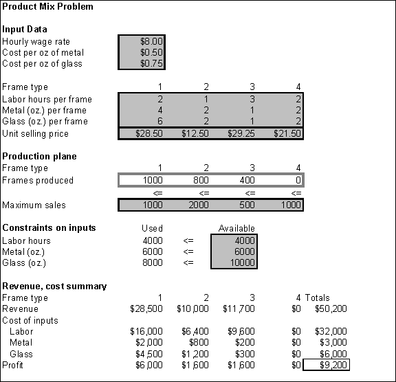
Overview: The Monet Company produces picture frames. The four types produced (1, 2, 3, and 4) are different in the areas of size, shape, and materials used. In addition, they require a certain amounts of skilled labor, metal, and glass as shown below.

Monet Picture Frame Data
	Skilled Labor	Metal	Glass	Selling Price
Frame 1	2	4	6	$28.50
Frame 2	1	2	2	$12.50
Frame 3	3	1	1	$29.25
Frame 4	2	2	2	$21.50

Next week, Monet can purchase up to 4000 hours of skilled labor, 6000 ounces of metal, and 10,000 ounces of glass. The associated unit costs are $8.00 per labor hour, $0.50 per ounce of metal, and $0.75 per ounce of glass. Production is subject to several market constraints that make it impossible to sell more than 1000 type 1 frames, 2000 type 2 frames, 500 type 3 frames, and 1000 type 4 frames.

Objective: Monet wants to maximize its weekly profit.

Decision and External Variables: The decision variables are the numbers of frames of type 1, 2, 3 and 4 to produce. The variables are labels x1, x2, x3 and x4. The external variables are hourly wage rate, cost per ounce of metal, and cost per ounce of glass.

Algebraic Formulation: Total profit and the constraints are written in terms of x as shown below. Explicit constraints are added to ensure that the x’s are nonnegative since only nonnegative amounts can be produced. Since the unit profits for each frame is $2, $6, $4, and $3, the profit objective statement shows the factor of profit for each frame. For each constraint, the left side states the factor for each product and the right side lists the maximum amount for each unit cost. Additional statements include maximum sales constraints and non-negativity constraints that put upper and lower limits on the quantities that can be produced.

LHS RHS
Maximize 6x₁ + 2x₂ + 4x₃ + 3x₄ Profit Objective
Subject to 2x₁ + x₂ + 3x₃ + 2x_{4 <=} 4000 Labor Constraint
4x₁ + 2x₂ + x₃ + 2x_{4 <=} 4000 Metal Constraint
6x₁ + 2x₂ + x₃ + 2x_{4 <=} 4000 Glass Constraint
x_{1 <=}1000 Frame 1 Sales Constraint
x_{2 <=} 2000 Frame 2 Sales Constraint
x_{3 <=} 500 Frame 3 Sales Constraint
x_{4 <=} 1000 Frame 4 Sales Constraint
x_1, x_2, x_3, x_{4 >=} 0 Frame 3 Sales Constraint

Spreadsheet Model: The spreadsheet model was developed using the steps below.

1. Enter the inputs. This data should be number taken directly from the problem statement.

2. Enter any four values in the range named Produced (frames produced for each frame type). Since these are the decision variables, Solver will find the optimal values.

3. Enter the formula =SUMPRODUCT(B9:E9,Produced) in cell B21 and copy to the rest of the Used range (amount of labor hours, metal, and glass used). This formula will calculate the units of labor, metal, and glass used by the current product mix.

4. To calculate revenues, enter the formula =B12*B16 in cell B27 and copy to the range C27:E27. To calculate costs, enter the formula =$B4*B$16*B9 in cell B29 and copy to range B29:E31. To calculate profits for each product, enter the formula =B27-SUM(B29:B31) in cell B32 and copy to the range C32:E32. To calculate the totals in column F, sum across each row using the SUM function.

Analyses
To use Solver to find the optimal solutions, select the Tools/Solver menu item. First, select the TotProfit cell as the target cell and click the Maximize button. Next, select the Produced range (number of frames 1-4 produced) as the changing cells. Finally, click on the Add button to add two constraints: Used<=Available and Produced<=MaxSales. The first constraint states that Monet cannot use any more of labor, metal, and glass than is available. The second constraint states that Monet cannot produce any more of each frame than can be sold. To make the changing cells nonnegative, add the additional constraint of Produced>=0. Since this model is linear, check the Assume Linear Model in the options dialog box. To find the optimal solution, click on the Solve button. Solver now searches all possible solutions until the optimal solution is discovered. At this point, the values generated by Solver can be retained. To keep the Solver solution, click OK.

Recommendations
Results from Solver indicate that the optimal action is to produce the following:

§ 1,000 Type 1 frames

§ 800 Type 2 frames

§ 400 Type 3 frames

§ 0 Type 4 frames

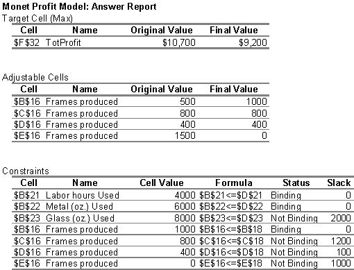
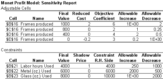
Although this is similar to Monet’s original production plan, Solver’s solution generates $450 more profit, using all of the available labor but only 80% of the available oz of glass. The following report shows that the constraints on the amount of labor hours, ounces of metal and ounces of glass used are “binding.” Since these constraints have 0 slack or are met exactly, they prevent Monet from earning a higher profit. Sensitivity analysis reveals that Monet can afford to pay and additional $1 per hour for labor to break even.

Click here to access the spreadsheet model